This article includes a list of general references, but it lacks sufficient corresponding inline citations. Please help to improve this article by introducing more precise citations. (October 2016) (Learn how and when to remove this message)

In the mathematical field of numerical analysis, interpolation is a type of estimation, a method of constructing (finding) new data points based on the range of a discrete set of known data points.^[1][2]

In engineering and science, one often has a number of data points, obtained by sampling or experimentation, which represent the values of a function for a limited number of values of the independent variable. It is often required to interpolate; that is, estimate the value of that function for an intermediate value of the independent variable.

A closely related problem is the approximation of a complicated function by a simple function. Suppose the formula for some given function is known, but too complicated to evaluate efficiently. A few data points from the original function can be interpolated to produce a simpler function which is still fairly close to the original. The resulting gain in simplicity may outweigh the loss from interpolation error and give better performance in calculation process.

Example

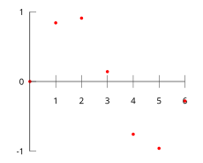
This table gives some values of an unknown function ${\displaystyle f(x)}$.

	${\displaystyle x}$		${\displaystyle f(x)}$
	0		0
	1		0	.	8415
	2		0	.	9093
	3		0	.	1411
	4		−0	.	7568
	5		−0	.	9589
	6		−0	.	2794

Interpolation provides a means of estimating the function at intermediate points, such as ${\displaystyle x=2.5.}$

We describe some methods of interpolation, differing in such properties as: accuracy, cost, number of data points needed, and smoothness of the resulting interpolant function.

Piecewise constant interpolation

The simplest interpolation method is to locate the nearest data value, and assign the same value. In simple problems, this method is unlikely to be used, as linear interpolation (see below) is almost as easy, but in higher-dimensional multivariate interpolation, this could be a favourable choice for its speed and simplicity.

Linear interpolation

One of the simplest methods is linear interpolation (sometimes known as lerp). Consider the above example of estimating f(2.5). Since 2.5 is midway between 2 and 3, it is reasonable to take f(2.5) midway between f(2) = 0.9093 and f(3) = 0.1411, which yields 0.5252.

Generally, linear interpolation takes two data points, say (x_a,y_a) and (x_b,y_b), and the interpolant is given by:

${\displaystyle y=y_{a}+\left(y_{b}-y_{a}\right){\frac {x-x_{a}}{x_{b}-x_{a}}}{\text{ at the point }}\left(x,y\right)}$

${\displaystyle {\frac {y-y_{a}}{y_{b}-y_{a}}}={\frac {x-x_{a}}{x_{b}-x_{a}}}}$

${\displaystyle {\frac {y-y_{a}}{x-x_{a}}}={\frac {y_{b}-y_{a}}{x_{b}-x_{a}}}}$

This previous equation states that the slope of the new line between ${\displaystyle (x_{a},y_{a})}$ and ${\displaystyle (x,y)}$ is the same as the slope of the line between ${\displaystyle (x_{a},y_{a})}$ and ${\displaystyle (x_{b},y_{b})}$

Linear interpolation is quick and easy, but it is not very precise. Another disadvantage is that the interpolant is not differentiable at the point x_k.

The following error estimate shows that linear interpolation is not very precise. Denote the function which we want to interpolate by g, and suppose that x lies between x_a and x_b and that g is twice continuously differentiable. Then the linear interpolation error is

${\displaystyle |f(x)-g(x)|\leq C(x_{b}-x_{a})^{2}\quad {\text{where}}\quad C={\frac {1}{8}}\max _{r\in }|g''(r)|.}$

In words, the error is proportional to the square of the distance between the data points. The error in some other methods, including polynomial interpolation and spline interpolation (described below), is proportional to higher powers of the distance between the data points. These methods also produce smoother interpolants.

Polynomial interpolation

Polynomial interpolation is a generalization of linear interpolation. Note that the linear interpolant is a linear function. We now replace this interpolant with a polynomial of higher degree.

Consider again the problem given above. The following sixth degree polynomial goes through all the seven points:

${\displaystyle f(x)=-0.0001521x^{6}-0.003130x^{5}+0.07321x^{4}-0.3577x^{3}+0.2255x^{2}+0.9038x.}$

Substituting x = 2.5, we find that f(2.5) = ~0.59678.

Generally, if we have n data points, there is exactly one polynomial of degree at most n−1 going through all the data points. The interpolation error is proportional to the distance between the data points to the power n. Furthermore, the interpolant is a polynomial and thus infinitely differentiable. So, we see that polynomial interpolation overcomes most of the problems of linear interpolation.

However, polynomial interpolation also has some disadvantages. Calculating the interpolating polynomial is computationally expensive (see computational complexity) compared to linear interpolation. Furthermore, polynomial interpolation may exhibit oscillatory artifacts, especially at the end points (see Runge's phenomenon).

Polynomial interpolation can estimate local maxima and minima that are outside the range of the samples, unlike linear interpolation. For example, the interpolant above has a local maximum at x ≈ 1.566, f(x) ≈ 1.003 and a local minimum at x ≈ 4.708, f(x) ≈ −1.003. However, these maxima and minima may exceed the theoretical range of the function; for example, a function that is always positive may have an interpolant with negative values, and whose inverse therefore contains false vertical asymptotes.

More generally, the shape of the resulting curve, especially for very high or low values of the independent variable, may be contrary to commonsense; that is, to what is known about the experimental system which has generated the data points. These disadvantages can be reduced by using spline interpolation or restricting attention to Chebyshev polynomials.

Spline interpolation

Linear interpolation uses a linear function for each of intervals . Spline interpolation uses low-degree polynomials in each of the intervals, and chooses the polynomial pieces such that they fit smoothly together. The resulting function is called a spline.

For instance, the natural cubic spline is piecewise cubic and twice continuously differentiable. Furthermore, its second derivative is zero at the end points. The natural cubic spline interpolating the points in the table above is given by

Zdroj:https://en.wikipedia.org?pojem=Interpolated
Text je dostupný za podmienok Creative Commons Attribution/Share-Alike License 3.0 Unported; prípadne za ďalších podmienok. Podrobnejšie informácie nájdete na stránke Podmienky použitia.

---