Cluster analysis or clustering is the task of grouping a set of objects in such a way that objects in the same group (called a cluster) are more similar (in some specific sense defined by the analyst) to each other than to those in other groups (clusters). It is a main task of exploratory data analysis, and a common technique for statistical data analysis, used in many fields, including pattern recognition, image analysis, information retrieval, bioinformatics, data compression, computer graphics and machine learning.

Cluster analysis refers to a family of algorithms and tasks rather than one specific algorithm. It can be achieved by various algorithms that differ significantly in their understanding of what constitutes a cluster and how to efficiently find them. Popular notions of clusters include groups with small distances between cluster members, dense areas of the data space, intervals or particular statistical distributions. Clustering can therefore be formulated as a multi-objective optimization problem. The appropriate clustering algorithm and parameter settings (including parameters such as the distance function to use, a density threshold or the number of expected clusters) depend on the individual data set and intended use of the results. Cluster analysis as such is not an automatic task, but an iterative process of knowledge discovery or interactive multi-objective optimization that involves trial and failure. It is often necessary to modify data preprocessing and model parameters until the result achieves the desired properties.

Besides the term clustering, there is a number of terms with similar meanings, including automatic classification, numerical taxonomy, botryology (from Greek: βότρυς 'grape'), typological analysis, and community detection. The subtle differences are often in the use of the results: while in data mining, the resulting groups are the matter of interest, in automatic classification the resulting discriminative power is of interest.

Cluster analysis was originated in anthropology by Driver and Kroeber in 1932^[1] and introduced to psychology by Joseph Zubin in 1938^[2] and Robert Tryon in 1939^[3] and famously used by Cattell beginning in 1943^[4] for trait theory classification in personality psychology.

Definition

The notion of a "cluster" cannot be precisely defined, which is one of the reasons why there are so many clustering algorithms.^[5] There is a common denominator: a group of data objects. However, different researchers employ different cluster models, and for each of these cluster models again different algorithms can be given. The notion of a cluster, as found by different algorithms, varies significantly in its properties. Understanding these "cluster models" is key to understanding the differences between the various algorithms. Typical cluster models include:

• Connectivity models: for example, hierarchical clustering builds models based on distance connectivity.
• Centroid models: for example, the k-means algorithm represents each cluster by a single mean vector.
• Distribution models: clusters are modeled using statistical distributions, such as multivariate normal distributions used by the expectation-maximization algorithm.
• Density models: for example, DBSCAN and OPTICS defines clusters as connected dense regions in the data space.
• Subspace models: in biclustering (also known as co-clustering or two-mode-clustering), clusters are modeled with both cluster members and relevant attributes.
• Group models: some algorithms do not provide a refined model for their results and just provide the grouping information.
• Graph-based models: a clique, that is, a subset of nodes in a graph such that every two nodes in the subset are connected by an edge can be considered as a prototypical form of cluster. Relaxations of the complete connectivity requirement (a fraction of the edges can be missing) are known as quasi-cliques, as in the HCS clustering algorithm.
• Signed graph models: Every path in a signed graph has a sign from the product of the signs on the edges. Under the assumptions of balance theory, edges may change sign and result in a bifurcated graph. The weaker "clusterability axiom" (no cycle has exactly one negative edge) yields results with more than two clusters, or subgraphs with only positive edges.^[6]
• Neural models: the most well-known unsupervised neural network is the self-organizing map and these models can usually be characterized as similar to one or more of the above models, and including subspace models when neural networks implement a form of Principal Component Analysis or Independent Component Analysis.

A "clustering" is essentially a set of such clusters, usually containing all objects in the data set. Additionally, it may specify the relationship of the clusters to each other, for example, a hierarchy of clusters embedded in each other. Clusterings can be roughly distinguished as:

• Hard clustering: each object belongs to a cluster or not
• Soft clustering (also: fuzzy clustering): each object belongs to each cluster to a certain degree (for example, a likelihood of belonging to the cluster)

There are also finer distinctions possible, for example:

• Strict partitioning clustering: each object belongs to exactly one cluster
• Strict partitioning clustering with outliers: objects can also belong to no cluster; in which case they are considered outliers
• Overlapping clustering (also: alternative clustering, multi-view clustering): objects may belong to more than one cluster; usually involving hard clusters
• Hierarchical clustering: objects that belong to a child cluster also belong to the parent cluster
• Subspace clustering: while an overlapping clustering, within a uniquely defined subspace, clusters are not expected to overlap

Algorithms

As listed above, clustering algorithms can be categorized based on their cluster model. The following overview will only list the most prominent examples of clustering algorithms, as there are possibly over 100 published clustering algorithms. Not all provide models for their clusters and can thus not easily be categorized. An overview of algorithms explained in Wikipedia can be found in the list of statistics algorithms.

There is no objectively "correct" clustering algorithm, but as it was noted, "clustering is in the eye of the beholder."^[5] The most appropriate clustering algorithm for a particular problem often needs to be chosen experimentally, unless there is a mathematical reason to prefer one cluster model over another. An algorithm that is designed for one kind of model will generally fail on a data set that contains a radically different kind of model.^[5] For example, k-means cannot find non-convex clusters.^[5] Most traditional clustering methods assume the clusters exhibit a spherical, elliptical or convex shape.^[7]

Connectivity-based clustering (hierarchical clustering)

Connectivity-based clustering, also known as hierarchical clustering, is based on the core idea of objects being more related to nearby objects than to objects farther away. These algorithms connect "objects" to form "clusters" based on their distance. A cluster can be described largely by the maximum distance needed to connect parts of the cluster. At different distances, different clusters will form, which can be represented using a dendrogram, which explains where the common name "hierarchical clustering" comes from: these algorithms do not provide a single partitioning of the data set, but instead provide an extensive hierarchy of clusters that merge with each other at certain distances. In a dendrogram, the y-axis marks the distance at which the clusters merge, while the objects are placed along the x-axis such that the clusters don't mix.

Connectivity-based clustering is a whole family of methods that differ by the way distances are computed. Apart from the usual choice of distance functions, the user also needs to decide on the linkage criterion (since a cluster consists of multiple objects, there are multiple candidates to compute the distance) to use. Popular choices are known as single-linkage clustering (the minimum of object distances), complete linkage clustering (the maximum of object distances), and UPGMA or WPGMA ("Unweighted or Weighted Pair Group Method with Arithmetic Mean", also known as average linkage clustering). Furthermore, hierarchical clustering can be agglomerative (starting with single elements and aggregating them into clusters) or divisive (starting with the complete data set and dividing it into partitions).

These methods will not produce a unique partitioning of the data set, but a hierarchy from which the user still needs to choose appropriate clusters. They are not very robust towards outliers, which will either show up as additional clusters or even cause other clusters to merge (known as "chaining phenomenon", in particular with single-linkage clustering). In the general case, the complexity is ${\displaystyle {\mathcal {O}}(n^{3})}$ for agglomerative clustering and ${\displaystyle {\mathcal {O}}(2^{n-1})}$ for divisive clustering,^[8] which makes them too slow for large data sets. For some special cases, optimal efficient methods (of complexity ${\displaystyle {\mathcal {O}}(n^{2})}$) are known: SLINK^[9] for single-linkage and CLINK^[10] for complete-linkage clustering.

• Linkage clustering examples
• 
  Single-linkage on Gaussian data. At 35 clusters, the biggest cluster starts fragmenting into smaller parts, while before it was still connected to the second largest due to the single-link effect.
• 
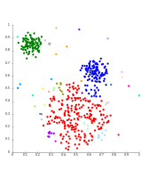
  Single-linkage on density-based clusters. 20 clusters extracted, most of which contain single elements, since linkage clustering does not have a notion of "noise".

Centroid-based clustering

In centroid-based clustering, each cluster is represented by a central vector, which is not necessarily a member of the data set. When the number of clusters is fixed to k, k-means clustering gives a formal definition as an optimization problem: find the k cluster centers and assign the objects to the nearest cluster center, such that the squared distances from the cluster are minimized.

The optimization problem itself is known to be NP-hard, and thus the common approach is to search only for approximate solutions. A particularly well-known approximate method is Lloyd's algorithm,^[11] often just referred to as "k-means algorithm" (although another algorithm introduced this name). It does however only find a local optimum, and is commonly run multiple times with different random initializations. Variations of k-means often include such optimizations as choosing the best of multiple runs, but also restricting the centroids to members of the data set (k-medoids), choosing medians (k-medians clustering), choosing the initial centers less randomly (k-means++) or allowing a fuzzy cluster assignment (fuzzy c-means).

Most k-means-type algorithms require the number of clusters – k – to be specified in advance, which is considered to be one of the biggest drawbacks of these algorithms. Furthermore, the algorithms prefer clusters of approximately similar size, as they will always assign an object to the nearest centroid. This often leads to incorrectly cut borders of clusters (which is not surprising since the algorithm optimizes cluster centers, not cluster borders).

K-means has a number of interesting theoretical properties. First, it partitions the data space into a structure known as a Voronoi diagram. Second, it is conceptually close to nearest neighbor classification, and as such is popular in machine learning. Third, it can be seen as a variation of model-based clustering, and Lloyd's algorithm as a variation of the Expectation-maximization algorithm for this model discussed below.

• k-means clustering examples
• 
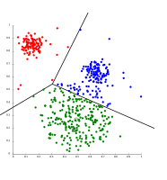  k-means separates data into Voronoi cells, which assumes equal-sized clusters (not adequate here).
• 
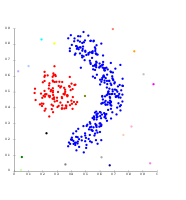
  k-means cannot represent density-based clusters.

Centroid-based clustering problems such as k-means and k-medoids are special cases of the uncapacitated, metric facility location problem, a canonical problem in the operations research and computational geometry communities. In a basic facility location problem (of which there are numerous variants that model more elaborate settings), the task is to find the best warehouse locations to optimally service a given set of consumers. One may view "warehouses" as cluster centroids and "consumer locations" as the data to be clustered. This makes it possible to apply the well-developed algorithmic solutions from the facility location literature to the presently considered centroid-based clustering problem.

Model-based clustering

The clustering framework most closely related to statistics is model-based clustering, which is based on distribution models. This approach models the data as arising from a mixture of probability distributions. It has the advantages of providing principled statistical answers to questions such as how many clusters there are, what clustering method or model to use, and how to detect and deal with outliers.

While the theoretical foundation of these methods is excellent, they suffer from overfitting unless constraints are put on the model complexity. A more complex model will usually be able to explain the data better, which makes choosing the appropriate model complexity inherently difficult. Standard model-based clustering methods include more parsimonious models based on the eigenvalue decomposition of the covariance matrices, that provide a balance between overfitting and fidelity to the data.

One prominent method is known as Gaussian mixture models (using the expectation-maximization algorithm). Here, the data set is usually modeled with a fixed (to avoid overfitting) number of Gaussian distributions that are initialized randomly and whose parameters are iteratively optimized to better fit the data set. This will converge to a local optimum, so multiple runs may produce different results. In order to obtain a hard clustering, objects are often then assigned to the Gaussian distribution they most likely belong to; for soft clusterings, this is not necessary.

Distribution-based clustering produces complex models for clusters that can capture correlation and dependence between attributes. However, these algorithms put an extra burden on the user: for many real data sets, there may be no concisely defined mathematical model (e.g. assuming Gaussian distributions is a rather strong assumption on the data).

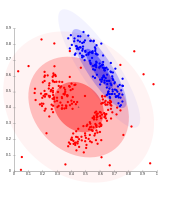
• Gaussian mixture model clustering examples
• 
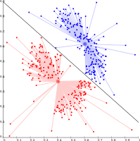
  On Gaussian-distributed data, EM works well, since it uses Gaussians for modelling clusters.
• 
  Density-based clusters cannot be modeled using Gaussian distributions.

Density-based clustering

In density-based clustering,^[12] clusters are defined as areas of higher density than the remainder of the data set. Objects in sparse areas – that are required to separate clusters – are usually considered to be noise and border points.

The most popular^[13] density-based clustering method is DBSCAN.^[14] In contrast to many newer methods, it features a well-defined cluster model called "density-reachability". Similar to linkage-based clustering, it is based on connecting points within certain distance thresholds. However, it only connects points that satisfy a density criterion, in the original variant defined as a minimum number of other objects within this radius. A cluster consists of all density-connected objects (which can form a cluster of an arbitrary shape, in contrast to many other methods) plus all objects that are within these objects' range. Another interesting property of DBSCAN is that its complexity is fairly low – it requires a linear number of range queries on the database – and that it will discover essentially the same results (it is deterministic for core and noise points, but not for border points) in each run, therefore there is no need to run it multiple times. OPTICS^[15] is a generalization of DBSCAN that removes the need to choose an appropriate value for the range parameter ${\displaystyle \varepsilon }$, and produces a hierarchical result related to that of linkage clustering. DeLi-Clu,^[16] Density-Link-Clustering combines ideas from single-linkage clustering and OPTICS, eliminating the ${\displaystyle \varepsilon }$ parameter entirely and offering performance improvements over OPTICS by using an R-tree index.

The key drawback of DBSCAN and OPTICS is that they expect some kind of density drop to detect cluster borders. On data sets with, for example, overlapping Gaussian distributions – a common use case in artificial data – the cluster borders produced by these algorithms will often look arbitrary, because the cluster density decreases continuously. On a data set consisting of mixtures of Gaussians, these algorithms are nearly always outperformed by methods such as EM clustering that are able to precisely model this kind of data.

Mean-shift is a clustering approach where each object is moved to the densest area in its vicinity, based on kernel density estimation. Eventually, objects converge to local maxima of density. Similar to k-means clustering, these "density attractors" can serve as representatives for the data set, but mean-shift can detect arbitrary-shaped clusters similar to DBSCAN. Due to the expensive iterative procedure and density estimation, mean-shift is usually slower than DBSCAN or k-Means. Besides that, the applicability of the mean-shift algorithm to multidimensional data is hindered by the unsmooth behaviour of the kernel density estimate, which results in over-fragmentation of cluster tails.^[16]

• Density-based clustering examples
• 
  Density-based clustering with DBSCAN
• 
  DBSCAN assumes clusters of similar density, and may have problems separating nearby clusters.
• 
  OPTICS is a DBSCAN variant, improving handling of different densities clusters.

Grid-based clustering

The grid-based technique is used for a multi-dimensional data set.^[17] In this technique, we create a grid structure, and the comparison is performed on grids (also known as cells). The grid-based technique is fast and has low computational complexity. There are two types of grid-based clustering methods: STING and CLIQUE. Steps involved in grid-based clustering algorithm are:

1. Divide data space into a finite number of cells.
2. Randomly select a cell ‘c’, where c should not be traversed beforehand.
3. Calculate the density of ‘c’
4. If the density of ‘c’ greater than threshold density
   1. Mark cell ‘c’ as a new cluster
   2. Calculate the density of all the neighbors of ‘c’
   3. If the density of a neighboring cell is greater than threshold density then, add the cell in the cluster and repeat steps 4.2 and 4.3 till there is no neighbor with a density greater than threshold density.
5. Repeat steps 2,3 and 4 till all the cells are traversed.
6. Stop.

Recent developments

In recent years, considerable effort has been put into improving the performance of existing algorithms.^[18][19] Among them are CLARANS,^[20] and BIRCH.^[21] With the recent need to process larger and larger data sets (also known as big data), the willingness to trade semantic meaning of the generated clusters for performance has been increasing. This led to the development of pre-clustering methods such as canopy clustering, which can process huge data sets efficiently, but the resulting "clusters" are merely a rough pre-partitioning of the data set to then analyze the partitions with existing slower methods such as k-means clustering.

For high-dimensional data, many of the existing methods fail due to the curse of dimensionality, which renders particular distance functions problematic in high-dimensional spaces. This led to new clustering algorithms for high-dimensional data that focus on subspace clustering (where only some attributes are used, and cluster models include the relevant attributes for the cluster) and correlation clustering that also looks for arbitrary rotated ("correlated") subspace clusters that can be modeled by giving a correlation of their attributes.^[22] Examples for such clustering algorithms are CLIQUE^[23] and SUBCLU.^[24]

Ideas from density-based clustering methods (in particular the DBSCAN/OPTICS family of algorithms) have been adapted to subspace clustering (HiSC,^[25] hierarchical subspace clustering and DiSH^[26]) and correlation clustering (HiCO,^[27] hierarchical correlation clustering, 4C^[28] using "correlation connectivity" and ERiC^[29] exploring hierarchical density-based correlation clusters).

Several different clustering systems based on mutual information have been proposed. One is Marina Meilă's variation of information metric;^[30] another provides hierarchical clustering.^[31] Using genetic algorithms, a wide range of different fit-functions can be optimized, including mutual information.^[32] Also belief propagation, a recent development in computer science and statistical physics, has led to the creation of new types of clustering algorithms.^[33]

Evaluation and assessment

Evaluation (or "validation") of clustering results is as difficult as the clustering itself.^[34] Popular approaches involve "internal" evaluation, where the clustering is summarized to a single quality score, "external" evaluation, where the clustering is compared to an existing "ground truth" classification, "manual" evaluation by a human expert, and "indirect" evaluation by evaluating the utility of the clustering in its intended application.^[35]

Internal evaluation measures suffer from the problem that they represent functions that themselves can be seen as a clustering objective. For example, one could cluster the data set by the Silhouette coefficient; except that there is no known efficient algorithm for this. By using such an internal measure for evaluation, one rather compares the similarity of the optimization problems,^[35] and not necessarily how useful the clustering is.

External evaluation has similar problems: if we have such "ground truth" labels, then we would not need to cluster; and in practical applications we usually do not have such labels. On the other hand, the labels only reflect one possible partitioning of the data set, which does not imply that there does not exist a different, and maybe even better, clustering.

Neither of these approaches can therefore ultimately judge the actual quality of a clustering, but this needs human evaluation,^[35] which is highly subjective. Nevertheless, such statistics can be quite informative in identifying bad clusterings,^[36] but one should not dismiss subjective human evaluation.^[36]

Internal evaluation

When a clustering result is evaluated based on the data that was clustered itself, this is called internal evaluation. These methods usually assign the best score to the algorithm that produces clusters with high similarity within a cluster and low similarity between clusters. One drawback of using internal criteria in cluster evaluation is that high scores on an internal measure do not necessarily result in effective information retrieval applications.^[37] Additionally, this evaluation is biased towards algorithms that use the same cluster model. For example, k-means clustering naturally optimizes object distances, and a distance-based internal criterion will likely overrate the resulting clustering.

Therefore, the internal evaluation measures are best suited to get some insight into situations where one algorithm performs better than another, but this shall not imply that one algorithm produces more valid results than another.^[5] Validity as measured by such an index depends on the claim that this kind of structure exists in the data set. An algorithm designed for some kind of models has no chance if the data set contains a radically different set of models, or if the evaluation measures a radically different criterion.^[5] For example, k-means clustering can only find convex clusters, and many evaluation indexes assume convex clusters. On a data set with non-convex clusters neither the use of k-means, nor of an evaluation criterion that assumes convexity, is sound.

More than a dozen of internal evaluation measures exist, usually based on the intuition that items in the same cluster should be more similar than items in different clusters.^{[38]: 115–121} For example, the following methods can be used to assess the quality of clustering algorithms based on internal criterion:

• Davies–Bouldin index

The Davies–Bouldin index can be calculated by the following formula:

${\displaystyle DB={\frac {1}{n}}\sum _{i=1}^{n}\max _{j\neq i}\left({\frac {\sigma _{i}+\sigma _{j}}{d(c_{i},c_{j})}}\right)}$

where n is the number of clusters, ${\displaystyle c_{i}}$ is the centroid of cluster ${\displaystyle i}$, ${\displaystyle \sigma _{i}}$ is the average distance of all elements in cluster ${\displaystyle i}$ to centroid ${\displaystyle c_{i}}$, and $$Zdroj:https://en.wikipedia.org?pojem=Cluster_analysis
Text je dostupný za podmienok Creative Commons Attribution/Share-Alike License 3.0 Unported; prípadne za ďalších podmienok. Podrobnejšie informácie nájdete na stránke Podmienky použitia.

---